- Visibility 129 Views
- Downloads 41 Downloads
- Permissions
- DOI 10.18231/j.ijashnb.2024.020
-
CrossMark

Brain tumor segmentation network: A study through interactive image selection and neural-nets training method
Abstract
Medical image segmentation is a pertinent issue, with deep learning being a leading solution. However, the demand for a substantial number of fully annotated images for training extensive models can be a hurdle, particularly for applications with diverse images, such as brain tumors, which can manifest in various sizes and shapes. In contrast, the recent Feature Learning from Image Markers (FLIM) methodology, which incorporates an expert in the learning process, has proven to be effective. This approach generates compact networks requiring only a few images to train the convolutional layers without backpropagation. In our study, we implement the interactive—technique for image collection plus neural-nets-training with reference to F.L.I.M, exploring the user’s knowledge. The results underscore the efficacy of our methodology, as we were able to select a small set of images to train the encoder of a U-shaped network, achieving performance on par with manual selection and even surpassing the same U-shaped network trained by backpropagation with all training images. Index Terms—Deep Learning, Brain, Tumor, Segmentation, Interactive Machine Learning.
Introduction
The gliomas are common brain tumors in grown-up-adults, with the Glioblastoma (GBM) being the commonest fatal brain—tumor of the CNS. In 2018-2019, the survival rate within 5 years following the diagnosis(diagnostic-findings) was 7% only, with an incidence rate of 2.55 per 100,000 people.[1]
The use of images is important for the initial diagnosis, with volume estimation essential for monitoring, investigat- ing tumor progression, and analyzing the selected treatment. However, manual annotation is time-consuming, tedious, and error-prone – facts that have motivated research on automatic and semi-automatic methods for brain tumor segmentation.
Two M.R.I/f-M.R.I sequences are employed mostly and commonly to capture brain/tumor sub-regions: Fluid Attenuated Inversion Recovery (T2-FLAIR or simply FLAIR) and the post-gadolinium-based contrast administration T1 (T1Gd). GBMs generally have an irregular shape and size, with active vasogenic edema (ED) on FLAIR and the enhancing tumor (ET) highlighted on T1GD. In addition to ED and ET, a third sub-region can also be observed, the necrotic core (NC), typically as a non-active region in T1Gd, delimited by ET.
Deep Learning (DL) presents the best results among auto- matic Brain Tumor Segmentation (BTS) techniques. However, traditional DL training requires many fully labeled images to train extensive networks and deal with different tumor appear- ances and other problems, such as images ac- quired from different machines and configurations (e.g., slice thickness).
Dynamic(or functional) learning is one technique that tries to explain and resolve the enigma, i.e., issue of finding the minimum set of training images.[1], [2] However, the process is usually done with an already predefined model without relating to visual characteristics or criteria for such selection, for example, sampling images based on latent representations.
One way to make the process more appealing is to reduce the gap between the user knowledge and the learning loop, such as selecting images. However, to minimize the subjective aspect of that interaction, it is essential to have a recommendation based on objective criteria.[3] Therefore, the present work proposes a way of selecting images at the same time that we learn convolutional filters, differing from image selection methods such as dynamic-learning. We apply feature-learning as of image-markers(FLIM) approach, in which the user draws biomarkers (i.e., bio-signals signatures) over imageries, and the filters are learnt as of the computationally marked area-regions (zone-wise) without backpropagation.[4], [5]
We propose an interactive methodology that learnt teaches filters as of drawn markers with FLIM. Then, the user selects another image that fails based on the already learned filters and objective criterion. The experiments demonstrate that through the selected data obtains results consistent with manual selection and superior to the model trained with all images of the training set.
Related Work
Image selection
As said before, some works use the user only as the oracle of the annotation, where there is a mechanism for recommending or sampling data, and the user only annotates those samples without properly selecting them. For example, some works measure uncertainty as a Bayesian problem using a probabilistic model,[6], [7] and others estimate uncertainty using distances from data representations.[7], [8]
Conversely, in contrast various works brought more relevance to the user, closing the gap between selection and annotation. For example, in,[9] the authors pursued ways of recommending data linked to visual explanation, even if the user is still only in the annotation process. In others, the user is the basis of selecting and annotating the data, selecting the data according to specific criteria.[3] However, most of those works are related to training the entire network on each interaction.
Feature learning from image markers
The FLIM’s preceding mechanisms and workings have demonstrated that it is possible to use a reduced number of weakly labeled images (1-8) to learn a shallow feature extractor (1-3 layers) with a descriptive proce- dure while maintaining its performance compared to standard deep learning models. This reduces the human effort to mark representative class regions in fewer images. With each marked region as a candidate filter, FLIM learns convolutional filters directly from those marked regions.
However, most works use visual inspection for the im- age selection method, which can be subjective and time- consuming.[10], [11] Others used clustering methods and direct 2d projection of images but did so on 2d image datasets for classification and without extracting features from such images.[4], [12]
Or set a marked image limit. In this work, we limited the number of images to 8 for a comparison with.[11]
We employ the interactive image selection only for the first layer, using the already selected images and drawn markers from the FLIM step to train the remaining encoder’s layers.
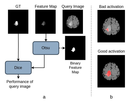
[Figure 2]. a presents the criterion used in the selection perfor- mance for a query image and feature map from one learned filter (a WT filter in this case). Otsu’s thresholding binarizes the activation map. The performance is measured by the Dice score between the ground truth (GT) and binary feature map. [Figure 2].b illustrates the process with examples of two acti- vations (after binarization), a ‘bad’ and a ‘good’ one. As the name suggests, the ‘bad’ activation misses parts of the tumor. However, we can generate the ‘good’ activation by selecting this image and learning filters from it. This ‘good’ activation is significant as it demonstrates the effectiveness of the learned filter in capturing a more substantial portion-of-tumor.
Materials and Methods
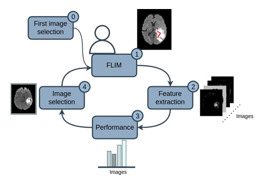
Our methodology followed the process in [Figure 1], where the user selects a first image (0), then marks relevant regions of the image and generates convolutional filters for the network encoder using FLIM (1). Such filters are applied to the remaining training images (2), and then a criterion is applied to obtain the performance of each remaining training image for these existing filters (3). Finally, in the next step, the user can select an image again (4), but now selecting the image with the worst performance given the established criterion.
Experiments
It is worth mentioning that during the FLIM process, the user annotates the convolutional filters between the regions of the brain that it detects (WT or ET). Then, the images performance are computationally done depending on those regions, and consequently user selects new images that fails depending on those regions. Finally, the image selection loop until all images perform well
Datasets
We used two datasets. The first is a private dataset con- taining 80 3D images of GBM with two MRI scans (FLAIR and T1Gd) per patient, and as a second dataset, we used the BraTS 2020 training dataset (293 samples), using the FLAIR- T1Gd pair.[13] For both datasets, we used the same preprocessing pipeline.[11]
We randomly divided the private dataset into 60% for imparting-training through the neural-nets, plus11% for the validation/verification, also30%for testing and executing and implementation. We kept the same amount of training data (50) for the BraTS dataset and separated the remainder between validation and testing (10/90%). We separated in this way to have a large set for testing, aiming to check whether the selection of images used can generalize well to the rest of the set.
Adopted architectural-design
For the architectural-design, we adopted a small 3D U-Net architecture, sU-Net, containing of 3convolutional-layer`s encoder and a symmetrical decoder.[11]
Encoder and decoder training
We use two learning methods: F.L.I.M to imparting and training the encoder and standard backpropagation to train the decoder. Among the 50 training images, we selected eight images by the interactive process of[Figure 1] and the rest of the 50 training images to train the decoder. For the backpropagation, we applied exact configuration of the learning rate and optimizer of.[11]
Evaluation metrics
We evaluate tumor segmentation into three regions: ET, Tumor Core (TC), and Whole Tumor (WT). The literature usually reports the segmentation effectiveness assuming that WT = ED ∪ ET ∪ NC and TC = ET ∪ NC. We applied Dice-Similarity-Coefficient (DSC) to measure efficacy.
Golden standard models
Deep Medic and nnU-Net models were used as golden standard models. These models adopt data augmentation, normalization, and learning rate reduction, providing us with upper-bound metrics. DeepMedic is a dual-branch network which was proved to use small amount of memory while maintaining performance,[14] and nnU-Net is a very relevant network, winning segmentation challenges of the last two years.[15], [16], [17]
Results
The table I presents the performance of the sU-Net model in the testing set with different image-selecting methods, either by applying all training imageries through the standard backpropagation, using FLIM with the user manually selecting the most diverse images for marking (F.L.I.Mm), and using the proposed interactive method (F.L.I.M.i). It is worth mentioning that the methods that used FLIM froze the encoder, so only the decoder was trained using backpropagation.
The table shows that the interactive method obtained the best mean values and lowest standard deviation, demonstrating the proposed method for selecting a diverse sub-sample of images for training. The interactive method saves the user time from manually selecting those images while reducing the subjective aspect of image selection. Also, our methodology based on FLIM outperforms the encoder trained with all training sets using backpropagation, as demonstrated within the Table—III for Bra-TS data set.
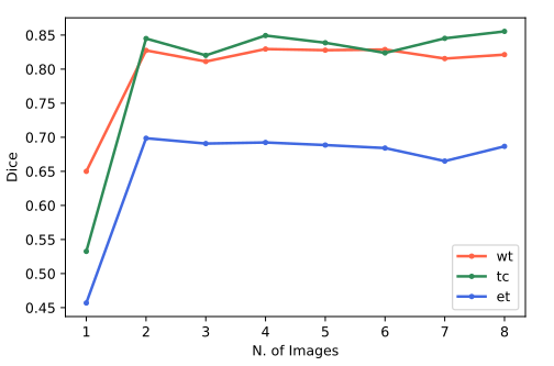
Furthermore, we verified the model’s performance for all ( ∀)for every new image which is selected and therefore marked, as shown in [Figure 3]. Note that there is a significant improvement when adding the second image (the first image is recommended). Also, for images 3-8, there`s no meaningful improve in the model’s performance, that is because of the first image being very typical and the second being very difficult, so the gains with the following images were small. The results also reinforce FLIM’s power in training encoders with very few images.
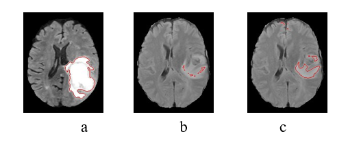
[Figure 4] shows the images from the first and second selec- tions, with the highlighted regions corresponding to the active regions for WT features. In (a), we have the image used on the first selection (i = 1) and the region of its best feature; in (b), we have the second marked image (i = 2) but with the best feature from the first – that doesn`t properly acquire the tumor, indicating why this image is recommended. In (c), the same image after training with F.L.I.M.
Note how attention improves from (b) to (c) by using this image with F.L.I.M. This visual improvement corresponds with the gains in the final segmentation (of sU-Net) for this specific image, going from a DSC of 0.01 to 0.65. This gain also corresponds to the gain of the image selection criteria of [Figure 2], which goes from 0.15 to 0.56.
We can correlate the final image metrics with its perfor- mance in the image selection criteria and the features learned in the first layer. Unfortunately, our criteria use the image’s GT, which prevents us from obtaining a reliable measure when making an inference from the test imagery which does`t have GT. Otherwise, this would be an excellent tool for using a system in clinical environments, providing not only the segmentation mask but also to which features it is related.
Next, we compare our trained model with the gold standard state-of-the-art models ([Table 2] ), with the neural-nets U-Net performing better, as expected. Yet, findings are nearly to such models, even using around 3% of the neural-nets/nn. U-Net parameters. Note that our goal is not to exceed such models since we use a much leaner network that trains fast (5% of neural-nets/nn. U-Net and 60% of Deep. Medic training time), but rather to obtain an estimate of how close (far) our results are to the ones of such massive networks.
|
Models |
|
||
|
ET |
TC |
WT |
|
|
Backpropagation |
0.665 ± 0.166 |
0.734 ± 0.157 |
0.721 ± 0.104 |
|
FLIMm |
0.691 ± 0.073 |
0.733 ± 0.072 |
0.702 ± 0.109 |
|
FLIMi |
0.713 ± 0.068 |
0.810 ± 0.066 |
0.797 ± 0.065 |
|
Models |
|
||
|
ET |
TC |
WT |
|
|
DeepMedic |
0.777 ± 0.056 |
0.851 ± 0.066 |
0.792 ± 0.094 |
|
nnU-Net |
0.798 ± 0.045 |
0.885 ± 0.058 |
0.851 ± 0.068 |
|
Ours |
0.713 ± 0.068 |
0.810 ± 0.066 |
0.797 ± 0.065 |
|
Models |
|
||
|
ET |
TC |
WT |
|
|
Deep Medic |
0.777 ± 0.175 |
0.810 ± 0.196 |
0.808 ± 0.138 |
|
nnU-Net |
0.842 ± 0.153 |
0.884 ± 0.163 |
0.906 ± 0.089 |
|
Ours |
0,717 ± 0,223 |
0,733 ± 0,237 |
0,789 ± 0,184 |
|
Backpropagation |
0,717 ± 0,214 |
0,734 ± 0,239 |
0,772 ± 0,184 |
Conclusion
Finding the smallest set-of-images that efficiently trains a network is a challenge. In the present work, we use a methodology that selects the training images while obtaining the convolutional filters from the encoder. The user draws markers on the selected images, learning convolutional filters from such markers. Then, the following training imageries can be selected according to the execution of the already learned filters. As a result, we selected a small set of images that trained the encoder of a U-shaped network, obtaining presentation analogous to manual selection and surpassing the accomplishment of neural-net-work imparted/trained with all available images. We wish to use the methodology for images of other nature in future work.
Source of Funding
None.
Conflict of Interest
None.
References
- Wu X, Xiao L, Sun Y, Zhang J, Ma T, He L. A survey of human-in-the-loop for machine learning. Future Gen Comp Syst. 2022;135:364-81. [Google Scholar]
- Mosqueira-Rey E. Human-in-the-loop machine learn- ing: A state of the art. Artif Intell Rev. 2023;56(4):3005-54. [Google Scholar]
- Zhao Z. Human-in-the-loop extraction of interpretable concepts in deep learning models. IEEE Transactions on Visualization and Computer Graphics. 2021;28(1):780-790. [Google Scholar]
- Benato B. Convolutional neural networks from image markers. . 2020. [Google Scholar]
- Souza I. Feature learning from image markers for object delineation. SIBGRAPI Conference on Graphics, Patterns and Images (SIBGRAPI). 2020. [Google Scholar]
- Wang Q. Deep bayesian active learning for learning to rank: a case study in answer selection. . 2021;34:5251-62. [Google Scholar]
- Li H, Yin Z. Attention, suggestion and annotation: a deep active learning framework for biomedical image segmentation. . 2020. [Google Scholar]
- Smailagic A, Costa P, Noh H, Walawalkar D, Khandelwal K, Agaldran M. Medal: Accurate and robust deep active learning for medical image analysis. . 2018. [Google Scholar]
- Uehara K, Nosato H, Murakawa M, Sakanashi H. Object detection in satellite images based on active learning utilizing visual explanation. . 2019. [Google Scholar]
- Sousa A, Reis F, Zerbini R, Comba J, Falca˜o A. Cnn filter learning from drawn markers for the detection of suggestive signs of covid-19 in ct images. . 2021. [Google Scholar]
- Cerqueira MA, Sprenger F, Teixeira BC, Falca˜o AX. Building brain tumor segmentation networks with user-assisted filter estimation and selection. . 2023;12567:202-11. [Google Scholar]
- Souza I, Falca˜o A. Learning cnn filters from user-drawn image markers for coconut-tree image classification, . . 2020;99:1-5. [Google Scholar]
- Kirby J, Burren Y, Porz N, Slotboom J, Wiest R. The multimodal brain tumor image segmentation benchmark (brats). IEEE transactions on medical imaging. 2014;34(10):1993-2024. [Google Scholar]
- Bakas S, Reyes M, Jakab A, Bauer S, Rempfler M, Crimi A. Identifying the Best Machine Learning Algorithms for Brain Tumor Segmentation, Progression Assessment, and Overall Survival Prediction in the BRATS Challenge. . 2018;3:1-49. [Google Scholar]
- Kamnitsas K, Ledig C, Newcombe V, Simpson J, Kane A, Menon K. Efficient multi-scale 3d cnn with fully connected crf for accurate brain lesion segmentation. Med Image Anal. 2017;36:61-78. [Google Scholar]
- Isensee F, Ja¨ger PF, Full PM, Vollmuth P, Hein KHM. nnu-net for brain tumor segmentation. . 2020;2020:118-32. [Google Scholar]
- Luu H, Park S. Extending nnunet for brain tumor segmen- tation, in Brainlesion: Glioma, Multiple Sclerosis, Stroke and Traumatic Brain Injuries: 7th International Workshop, BrainLes 2021, Held in Conjunction with MICCAI 2021, Virtual Event. . 2021. [Google Scholar]